|
| home resume portfolio |
| Yinsh Rez Advance Oil Painter |
Oil PainterContents | ||||||||||||
|
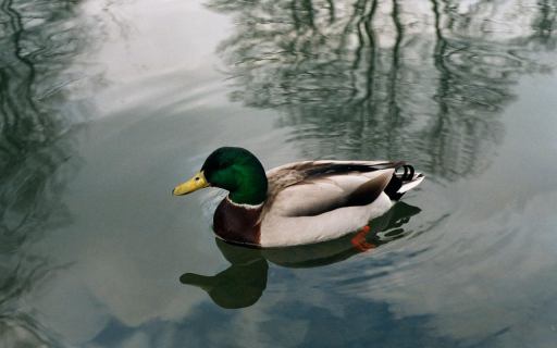
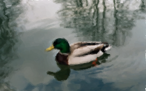
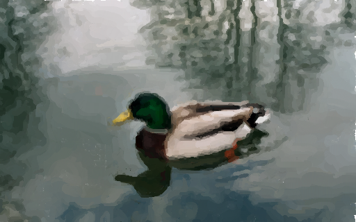
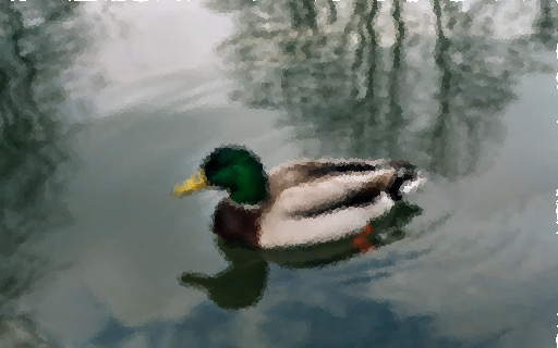
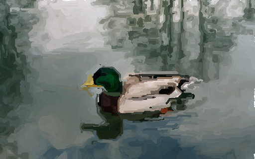
Background This oil painting program was my final project for my Computer Graphics class at the University of Waterloo. This project was based off the paper Painterly Rendering with Curved Brush Strokes of Multiple Sizes by Aaron Hertzmann. The program can take bitmap images and convert them to an oil painted version. As well, a simple 3D renderer and key-frame animator was created to make oil painted videos. | ||||||||||||
|
Top | ||||||||||||
Download
| ||||||||||||
|
Top | ||||||||||||
Screenshots
| ||||||||||||
|
Top | ||||||||||||
|
Design This project has two major components: the painting filter and the 3D animation engine. Painting Filter The painting algorithm simulates the use of brush strokes to generate an image. It uses a multi-pass algorithm with different brush stroke sizes, going from largest to smallest. This builds up the finished painting, with large brushes creating the general colour flow, moving down to the smaller brush strokes finer details. The algorithm starts with a blank canvas and an image to paint. The first step is to generate blurred versions of the image, with the blurring radius equal to the radius of the brushes to be used. I implement the blurring algorithm using a summed area table. The summed area table of an image has the value at the coordinates (x,y) of the sum of all the pixels in the rectangle with corners (0,0) and (x,y). This is computed in O(n) where n is the number of pixels. To generate a blurred image, using a linear blur, find the value of the rectangle with width and height 2*radius, around the pixel of interest. This can be calculated in constant time from the summed area table, so to generate the blurred image is also O(n). The Summed-Area Table is implemented as the SAT object found in the sat.cpp file. Start with the largest radius; compare the blurred image to canvas (which starts as blank). Divide the image into a grid, where the grid height and width are equal to the radius. Perform a summed squared difference in each grid, and compare it to a threshold value, if the error is greater than the threshold start a brush stroke in this spot. Each brush stroke is assigned a random z value so that the order of strokes is not regular. To do this, I add each stroke starting position to a priority queue, which I can then remove in order when I draw them. This is necessary to have the proper blending when using brush textures. This algorithm is implemented in Painter::paint. To generate the control points for the brush stroke, we want to follow perpendicular to the gradient of the image at the current point of the stroke. The brush stroke is given the colour of the blurred image at the starting point. A luminance map of the blurred image is used, calculated with 0.3*r + 0.59*g +0.11*b. A Sobel filter is used to calculate the gradient. I use the 3x3 matrices for horizontal and vertical gradient calculations. These give me the horizontal and vertical vectors of the gradient, which I use to calculate the perpendicular vector. I chose the perpendicular vector which has the smallest angle from the previous control point. Use this vector, with a magnitude equal to the radius, to find the next control point. For each new control point, compare the stroke colour with the pixel colour at that control point on the blurred image, if the difference between the two is greater than the difference between the stroke colour and the canvas, stop adding control points. Also, you can specify a minimum and maximum stroke length. Control points are stored in a vector, and the entire stroke is encapsulated in a class to both interpret the points and render the stroke. This part of the algorithm is implemented in Painter::genbrushstroke. Now that we have a set of control points, we want to turn them into a nice stroke. With a uniform spacing of the control points, we can interpret it using a cubic B-Spline subdivision algorithm. Fix the start and end points as the start and end control points, then add control points at the half way point between each 2 consecutive control points. Use three consecutive original control points, and the first derivative equation for a cubic B-Spline, to get the new coordinates for the middle control point. So for points p1, p2 and p3, the new coordinates for p2 are 1/6(p1 + 4*p2 + p3). Performing only 1 subdivision is all that’s necessary since the radius of the strokes will absorb any more subtle differences. Code for this can be found in Stroke::subdivide. The last step is to take this spline and draw it as a triangle strip. This can be done simply by calculating the vector between two control points, (consecutive at the ends, or the points surrounding a middle control point), and using the perpendicular vector to calculate the two coordinates around that control point on the triangle strip. The strip will have a diameter of 2 times the radius of the brush stroke. Capping the ends of the strip with triangle fans adds to a nice curved appearance. Finally, an alpha texture can be applied to the stroke to blend it in with the canvas or previous strokes. This will smooth the edges of the brush strokes giving a softer final image. Code for this can be found in Stroke::drawstroke. Finally, when all the strokes of one radius have been drawn, the resulting image is used as the canvas for the next set of smaller strokes. This means that the smaller strokes only will be painted in areas that are not accurately represented by the large brush. The combined layers of brush strokes create the finished image. Animated Paintings An extension to this algorithm is to update the brush strokes to reflect changes from the original image. Since brush strokes are drawn in a random order, just applying the filter to each frame in an animation will cause a lot of flickering in areas that are not changing. To solve this, we only want to paint new brush strokes where the image is changing. So for each new frame, calculate the difference between that frame and the one preceding it. Add this to a difference buffer. When the summed grid area of the difference buffer gets over a threshold, resent that grid to 0 and draw a brush stroke starting in that area. You can see this difference buffer at the start of Painter::paint. With this pre-calculation, you don’t need to calculate the summed squared error for grid spots that have not changed, speeding up the filter, and making the animated frame-rate faster than applying the filter to each frame as if it were a static image. Also, the finished painting from the previous frame can be used as the canvas for the next frame, helping to reduce the amount of new brush strokes to generate. 3D Animation Engine The other component to the project is the 3D animation engine. The main part of the engine is the key frame animator. The animator stores an ordered vector of frames and particle systems. There will be at most one active frame. That frame will can access the next frame, and use the start and end values to linearly interpolate position and rotation of models at any time t between itself and the next frame. There can be multiple particle systems active at any time t. Rending the particles happens in two phases. First all the particle positions are determined (based on the time t), and they are sent into a priority queue ordered by z coordinate. This means we can render them back to front, and allow the proper blending effects. Every rendering function is designed to work at a random time t, so that the animation can move forwards and backwards without issue. To calculate the linear interpolation, it’s simply: Position(t) = Position1 + (time – starttime)(Position2-Position1) For the particles, we need a quadratic equation to have acceleration come into effect: Position(t) = origin + time*velocity + time*time*accel*direction/2 where direction is the normalized velocity vector. Texture mapping on the meshes is accomplished using the glGenTex automatic texture coordinate generation system. For one texture, the plane is set to face one of the three axis, in either a positive or negative direction. For two and six textures, the dot product of the axis and the face normal is used to determine in which direction the face is facing. Then all the faces are pushed into a priority queue. Then each group of faces is removed and the texture coordinates are generated for that group of faces. Pixel Shader Optimizations The idea was to use the GPU to calculate the blurred images and perform the difference operation from the blurred images and the current canvas. The blurred images would be calculated using a linear blur, on a two pass system. First a horizontal blur, followed by a vertical blur. 5 overlapping but slightly offset textures would be summed to create the blurred image. The blurred images would then be combined with the current canvas, using a pixel shader that would compute the difference then sum the squares. The visual results from using the pixel shaders were equivalent to those from using the CPU equations. However, the performance was actually slower. I can see a few reasons for this. First, using the SAT to make 3 blurred images takes 4 passes over all the pixels. The pixel shaders require 6 passes, since for each level of blur, a horizontal blur and a vertical blur must occur. As well, it transfers 3 times as much information from the graphics memory to the system memory (each blurred image needs to be dumped to system memory). This transfer is relatively slow compared to simply working in system memory. However, these operations are stilled being done on the GPU, so theoretically, that should free up more CPU cycles. In a more complex program, those cycles could be used to do other computations while waiting for the GPU to finish its work. | ||||||||||||
|
Top | ||||||||||||
|
Source Code The Oil Painter was written in C++ using the Simple DirectMedia Layer Library and TinyXML parser. The code requires the OpenGL header files, and has been compiled on both Windows and Linux platforms.
| ||||||||||||
|
Top |